Did I Hear Somebody Say Reinforcement Learning?

Introduction

To explore, to compare and to learn - three core ideas of training a machine with RL. Instead of a person, we have an actor, also known as an agent, which is simulated in virtual reality. It's been a while since I wanted to talk about the things in reinforcement learning, and how they are connected. More about that in the text below!

TL;DR We're going to go over RL in general, then move to LLMs, then run experiments in this notebook training an LLM to detect hallucinations

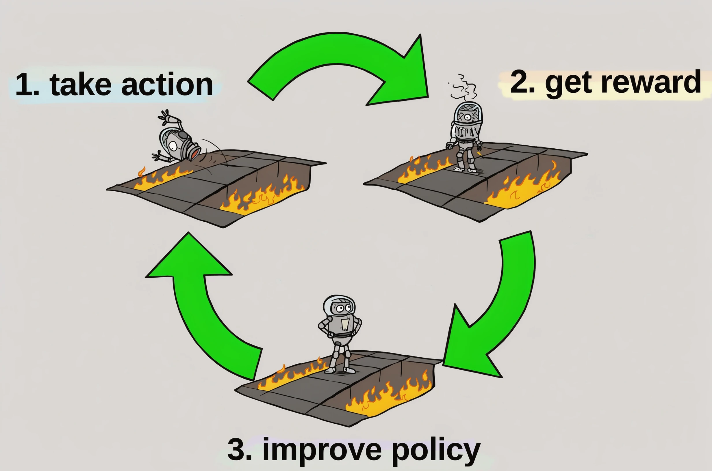
As in the image above, a small robot inside an environment is currently occupied with one goal - to get out of a burning corridor. Every time it tries, it gets to a new state within the broad situation. The realizations of the environment and of the robot's behavior in it can happen indefinitely at the speed of computations; planning and sampling the real environment's outcomes are what earn the robot rewards for its actions, and insights into how to act next. Through such a process we can train a robot to act according to the most optimal policy, in other words to have the agent implement the action playbook.

Most write-ups on RL start with Markov decision processes and classical statistical methods, then deep learning. I'm not going to be an exception here, and you can see what's coming in the table of contents.

Table of Contents

First, the classics. We'll:

• walk you through the MDP and its formalism;
• talk about advantage and value functions;
• skim through Q-learning with neural networks.

After that we move on to RL with LLMs:

• SFT vs RL
• PPO vs GRPO
• Dr.GRPO and GSPO

Practical part:

• introducing the problem that we can try to approach with RL
• training a text classifier that predicts whether text is hallucinated
• comparing the results from two approaches (QA vs summaries from the HaluEval dataset)
• sharing the code on AMD notebooks

System design section:

• Now we have a model, what's next?
• Serving it / making it available as an app
• Evaluating the QoS of your inference
• Touching upon the training infra

Markov Decision Process

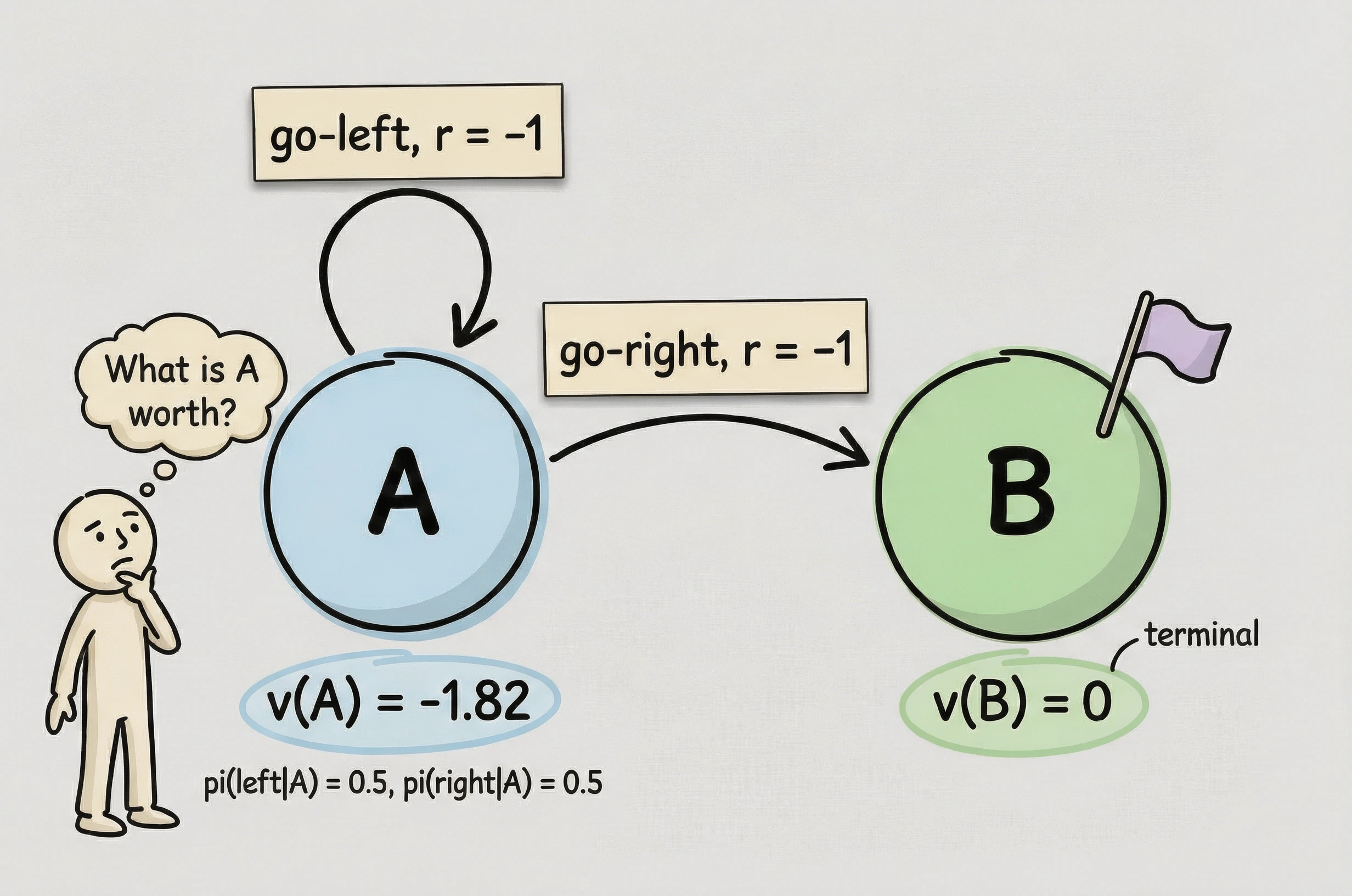
Above there's a graph of an MDP. We enter the environment in state A, we can go left and end up in the same spot, or go right and reach the terminal state.

Our reward is -1 (that's just by construction) no matter which decision we take in this very state. Our policy is to choose left half of the time, and right the other half. The value functions of the states are A = -1.82 and B = 0.

The value function is defined as:

where $\gamma$ is the discounting term.

So, in the case where $\gamma = 0.9$, the value function of state A is:

($v(A)$ appears on both sides of the equation because there's a cycle in the graph)

In RL with an MDP we optimize the value function, which helps us build the optimal path through the graph of states and actions. The value is defined recursively from the end state back to the start, and is usually solved as a dynamic programming task. In each state an immediate reward may be negative for all the actions, but the end-game value of some of them is higher than that of others; based on that we greedily select the most optimal policy for our agent.

In my opinion, authors tend to fall into one of two categories when they eventually lead their thoughts towards modern RL. They give you a skim over the fundamental approaches. Or they skip the historical note entirely and jump straight to the reinforcement learning of the reasoning traces of LLMs, often showing you the hands-on demo right away.

I propose that you look at this perspective, which has elements of both ends of the spectrum. We'll take a look at the code and run it, and we'll also get some intro to what the industry considers interesting from a theoretical perspective.

Round 1. Fight!

Advantage and value functions

Do you know the rules of Tic Tac Toe? You drop Xs and Os on a 3-by-3 board in the hope of outsmarting your opponent and drawing 3 in a row first. Or at least leading it to a tie.

The board with your opponent is an environment. Every turn you take on the board prompts your opponent to change the current state of the board before your next move. Each action has an end value, so let's formalize it.

Values tell us how good a board is. But when it's our turn, we don't choose boards; we choose moves. So the natural question is: how much does a move change our position?

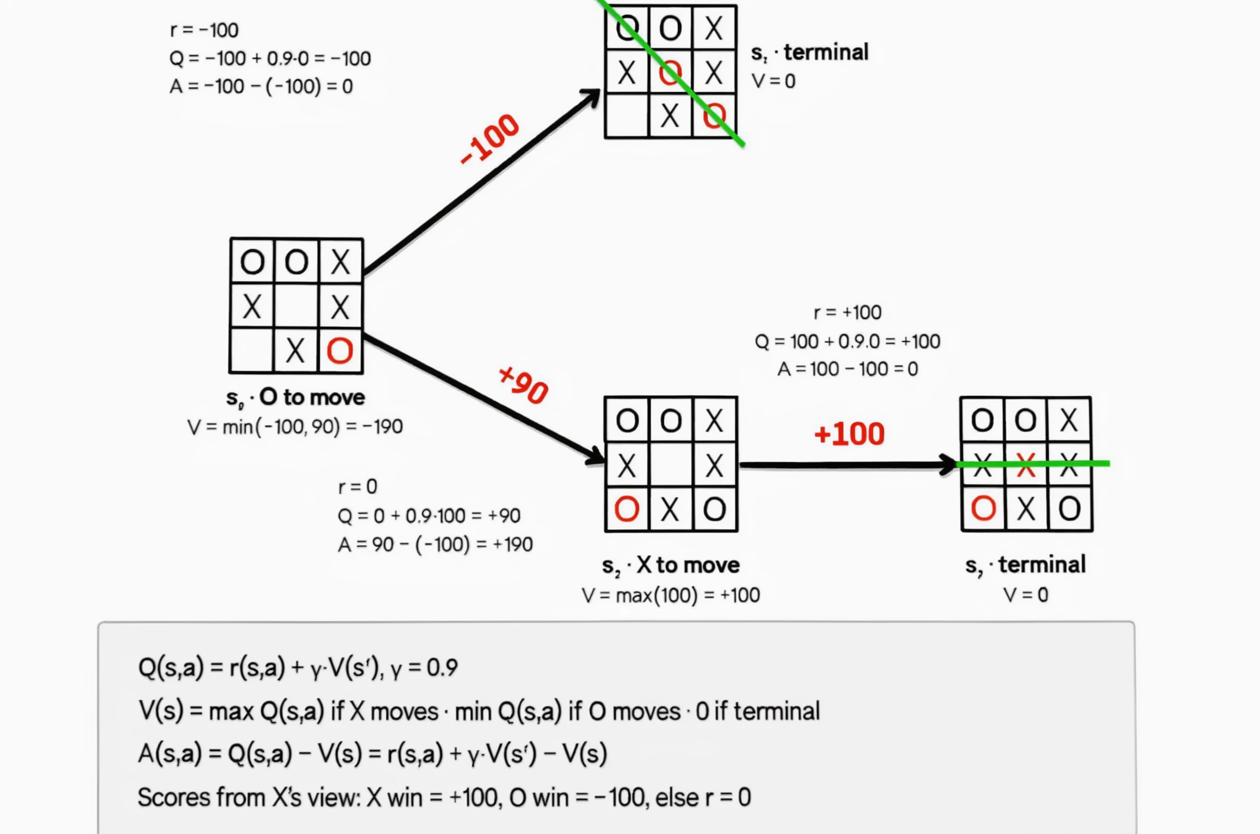
The top board is worth 0: with best play from both sides, the game ends in a draw. If O plays top-left, the next board is worth +1, a forced win for X. If O plays bottom-middle, the next board is still worth 0. Subtracting the value before the move from the value after it gives each move's advantage: +1 for top-left (a gift to X) and 0 for bottom-middle (which holds the draw).

Here's the formalization:

where $V(s)$ is the value function of the state variable, and $Q(s, a)$ is the Q-function of state and action.

The Q function belongs to a class that can be defined like this:

where $s$ and $s'$ are related as the previous and the following step, and $r(s,a)$ is the immediate reward function given an action.

So we might infer that some actions are more advantageous, and that earlier actions decide what the total outcome is going to be.

It doesn't ask "Is this position good?" It asks "Did this move make things better or worse than they already were?"

By training, we are trying to maximize the value function and find the argmax policy that achieves it:

where $a$ are the actions and $s$ is any given possible state.

HJB and optimal control

In the continuous case, where the state is a point in multi-dimensional real space, the new state translates to $s' \to x + f(x,u) \cdot \Delta t$, the current coordinate shifted by the dynamics function proportional to the time that has passed.

For example, a rocket is moving through space to bring a satellite there; it propels the load into space, and at the same time towards a certain point in space where the satellite should start, potentially with inherited speed as well.

The value function of such a case will look like this:

And here's the HJB itself

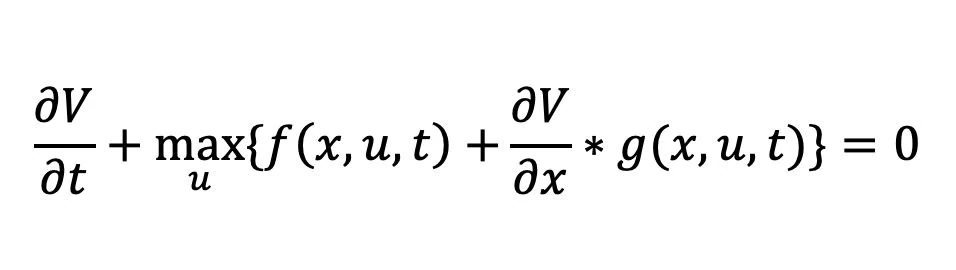
If you can solve the guy above for any optimal control problem, you're a total beast!

• $u$ is a control (the action): the thrust and direction the rocket can apply at state $x$. The control that achieves the max, $u^*(x)$, is the optimal control, and the rule $x \mapsto u^*(x)$ that gives it for every state is the optimal policy.
• $r(x,u)$ is the reward, or inverse losses (like fuel cost or burn rate)

Reinforcement Q-Learning (aka DQN)

My intro to RL was through an NN course hosted on the premises of MSU. While there, I tried to reproduce OpenAI's results on the Atari games gym, the OG gym (openai/gym). I trained a model on my favorite game from the list, the arkanoid-style one called "Breakout!", and it was one of the few that are sort of continuous, in the sense that you position the carriage within a line; all the games in gym are real-time games.

So, if you want to control the carriage, you need to infer the rollouts quickly - otherwise, GAME OVER

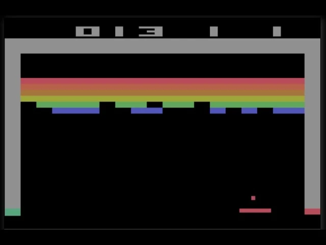
In DQN you train a network $Q_\theta(s, a)$ to satisfy the Bellman equation. The ingenuity of the math translated into a statistical method driven by machine learning, specifically deep learning.

While training a model I made an interesting observation at the time: to train such a model, the loss convergence happens only when you learn to predict actions for the fifth frame. My guess is that it had something to do with learning the dynamics of the game from those 4 frames in context; it needed three derivatives of everything on the game screen, meaning speed, acceleration and even jerk.

You can check out my old work here

NOTE: Some of the slides in this post are inspired by an amazing educational repo, which was originally maintained by fellows from Yandex, back in 2018 when Yandex used to be headquartered in the Netherlands. Check out the course Practical RL

So why RL at all?

Let's move from the simple gaming agent cases of reinforcement learning with deep neural networks closer to the state of things in the LLM space, or in any artificial intelligence model in 2026.

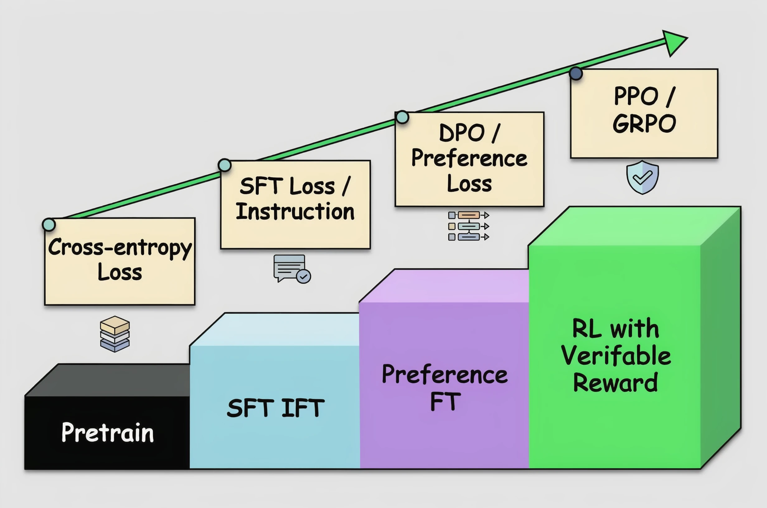
You want to improve your agent, which is the language model, to generate better outputs given your metrics. Each output token it gives is in some sense a selection from the discrete but huge space of possible continuations of the reply. The state and environment are dictated by the model policy and by what the world expects from the task.

The context defines the next token prediction, so you can adjust the probabilities of all tokens to be generated at any given step. Usually you derive the verifiable reward from a data source, and the model learns to do reasoning prior to putting out the predicted action / label / tool call, or just simply text.

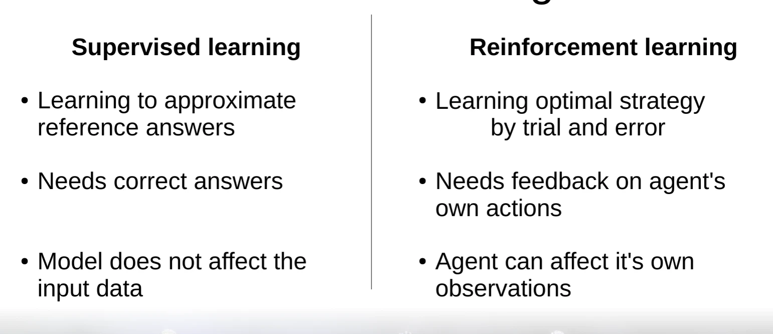
The constructed use case looks like this: you have the gold labels but no gold reasoning. SFT needs target completions. SFT maximizes token likelihood; RL optimizes the thing you score.

RL in LLMs

Why do we even bother with RL? Is it the only viable approach to training?

Here's the tipping point, when it first blew our minds: they trained ChatGPT-3.5 with SFT and RLHF, which stands for Reinforcement Learning with Human Feedback.

RLHF - what did it look like?

RLHF is a pipeline: you collect human preferences, fit a reward model on them, and then optimize your policy against that reward. PPO - proximal policy optimization - is the algorithm that does that last step, and it's the one that needs a separately trained critic alongside the policy. PPO was later replaced by GRPO, and the term came from the DeepSeekMath authors. In the labs of closed-source companies like OpenAI / Anthropic it might have had another name. GRPO does not require a critic trained separately; it can improve based on the advantages drawn from the same policy. That sounds too good to be true until you recall REINFORCE (yes, all caps, that's the right spelling): subtracting a baseline from the return leaves the policy gradient unbiased while reducing its variance. You pay nothing in correctness and get a much calmer gradient, and a group of rollouts for the same prompt is simply a cheap way to estimate that baseline.

PPO vs GRPO

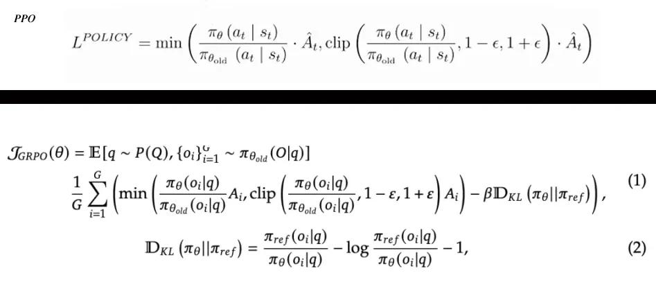
Here are the terms for PPO and GRPO

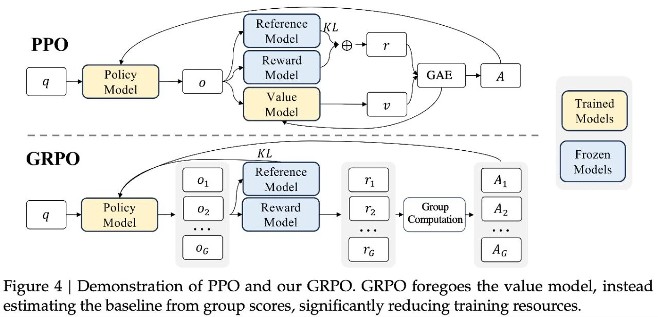
And as a data flow architecture

REINFORCE: we sample a completion, score it, and push up the log-probability of its tokens in proportion to the reward minus a baseline; no ratio, no clipping, no critic.

Proximal Policy Optimization: in this case we try to stay closer to the original policy when we do an update; this one introduces the importance sampling ratio; there's a critic model that we either already have or have to train.

Group Relative Policy Optimization (GRPO): we keep PPO's importance sampling ratio and clipping, but drop the critic; the advantage of each rollout is its reward compared to the other rollouts sampled for the same prompt (minus the group mean, divided by the group std).

Importance Sampling Ratio

At every step of the policy update we do it with regard to the initial policy pi_old and the current generated action. Pi_old sits in VRAM waiting, and it is of size (B, T), meaning batch of responses times max response length, type=Float32, requires_grad=False. The formula is

Reading it left to right: $q$ is the prompt and $o_{i,<t}$ is everything the $i$-th rollout has generated before position $t$ - together they are the state. $o_{i,t}$ is the token that was actually sampled there, which is our action. The forward pass $NN_\theta$ gives logits over the whole vocabulary, softmax turns them into a distribution, and the bracket at the end just picks out the one entry we care about. One scalar per token, which is why the cached tensor is (B, T).

That is one half of the ratio. The other half is the same number computed under $\pi_{old}$, and the ratio itself is simply

We need it because the rollouts came from the old policy, but the gradient we want belongs to the current one; the ratio pays for that mismatch and lets us take several optimizer steps on the same batch of samples. In code it lives in log space, exp(logp - logp_old), otherwise you underflow on the first token.

RLHF was one of the earliest examples of successful PPO on LLMs. In reinforcement learning with human feedback we use a critic model, a generative classifier that assigns a reward to each completion in the rollout based on the preferences from the expert-curated dataset.

Dr.GRPO and GSPO

Let me go over two options you might stumble upon when you explore the topic of GRPO further. GRPO has been proven inferior by a bunch of measures, e.g. MoE training stability or length bias. And if you use its vanilla version, you're probably going to spend more on a cloud bill than an optimized version would cost.

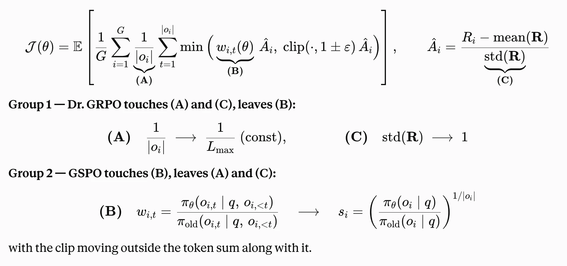
Dr.GRPO addresses the bias where short answers with a positive advantage were incentivized more than long ones and, vice versa, where the negative-advantage sequences were not penalized enough for high verbosity.

It introduces two adjustments to the main loss term, strict and simple:

• they scale the sum of advantages of the tokens in a rollout by the len of the longest trajectory we decide on beforehand, the same divisor for every rollout, instead of normalizing it individually by the len of each
• and they give up on dividing by std when computing the in-group advantage. Remember, REINFORCE's first optimization requires only the baseline subtracted from the local advantage.

GSPO introduces an improvement on a different axis, on a harder one: the importance sampling ratio itself.

The default Group Relative approach has proven unstable when we talk about the training of a mixture-of-experts model. Instead of a ratio per token, GSPO builds one ratio for the whole sequence - the likelihood of the entire completion under the current policy over its likelihood under pi_old, normalized by length so long and short rollouts stay comparable. The clipping then happens once, on that single number, so a rollout is inside the trust region or outside it as a whole rather than token by token. The gradient still reaches every token in the sequence; what changed is that all of them now share one weight instead of each carrying its own.

How would you design a system that requires RL?

1. Collecting requirements

Say we were to design a system which has RL as a solution, and our task is to train and serve such a model.

First you settle on the problem: what do they want to optimize - is it a language task or a vision task, probably language; what do they optimize for - perhaps they want to reduce the hallucinations of the LLM; do we know exactly what a hallucination looks like - maybe not, and we need to decide and define it on our own.

Secondly, what resources do we have to train a model? Are there any limitations on hosting the resulting model?

For example, we can go all in and rent a cluster from a datacenter (bare metal, somewhere far away). Or perhaps rent a machine from TogetherAI or Modal, or RunPod. There's an option to train your model with Tinker from ThinkingMachines; there you can train the model through configs and RL environments, no infra code required.

2. Research

Do research on the datasets, find the most relevant ones by description, rank them and look into the samples of the dataset. If, for example, we want to reduce the hallucinations of a financial advisor bot, we look for a financial terms dataset, perhaps one that contains trades or decisions made on an investing strategy. Or hallucinations in medical output - diagnosis writing, for example, or prescription writing. Say there's a summary of an anonymized visit between a patient and a doctor, and the doctor says in the text that the patient needs a certain ointment. The onboard intelligence might want to pass this prescription to the pharmacy in a specific format; violating such a format might be considered a hallucination by the pharmacist in the field.

3. Experiments

Start by securing compute; in my case I run Jupyter notebooks on a ~200GB AMD MI300X GPU. You have to fill in boilerplate code with training configuration, entity instantiation (trainers / loggers / dataset providers). You can follow my recent experiment code here; it's on Colab, but to run it you need ~140GB of memory.

I use trl, a library from HuggingFace. There we instantiate a trainer with a reward function. The reward function is actually the most important piece in the pipeline.

How do we distinguish whether generated text contains hallucinations or not? The idea is to move the token probabilities towards generating thinking traces, after which we predict the probability of a hallucination as the very last token.

NOTE: RL vs Self Distillation There's a caveat in between: self-distillation and reward, they possess some commonalities. In self-distillation we usually train to produce the most probable outcomes of the old model with more confidence. There's no reward function, but at the same time, like in RL, we sample from the model's own distribution and run several steps of backpropagation through the samples.

Below you can find the approximate prompts I use for the reward function; the full notebook you can see here.

The dataset we use consists of the following: there are prompts and responses from different LLMs, such as Gemini, GPT, and Claude. There are labels for each (prompt, response) pair - was it a hallucination, or was it a right answer. There are human labels with a justification, and automated LLM labels (synthetic data).

The RL prompt environment will look like this:

You are given a prompt completion pair, predict "Class: ...", where ans in [haluc, correct],

Prompt: {prompt}, with completion: {completion}

Knowledge: {knowledge}

<Justification>

Class: halucination (or class: correct)

For the first experiment we use Qwen2.5-3B-Instruct. We trim the last word from the output of decoded tokens from the neural network, and compare it against the ground-truth class; if it matches exactly we give such an action a full reward of 1.

We use the HaluEval dataset and the QA section of it with 10k items, where examples of hallucinated answers are balanced 50/50.

If our prompt contains valid knowledge, which in this case it does, then through the training the policy should be able to learn to assign probabilities to the class based on the knowledge, and to find contradictions with the answer if they differ factually.

The graph clearly shows that with such an approach we reach a far superior f1 score to naively predicting "halluc" all the time - in that case precision would be 0.5 and recall 1.0, thus f1=66.6%; we have almost 90% on train and val.

Such an approach is not very useful to an end consumer; such a classifier would be rendered useless in cases where we don't have any knowledge (we could pull up some from a search engine though!).

If we drop the "Knowledge" from the visible prompt, the model stops learning anything useful from the input.

Perhaps we should train something with paired data: each hallucinated and correct response alongside the input question. Now we have:

Question: {prompt}
Response: {response_correct | response_false}

<Justification>

Class: {"hallucination" | "correct"}

For some reason, with such an approach we almost instantly saturate to non-informative zero_std in advantages. We should try a more capable model: Qwen2.5-3B-Instruct -> Qwen3-4B (one could try to use -4B-Instruct-2507). And indeed, after the switch to the more capable Qwen3-4B we see that there's no gradient starvation: zero_std after the first fifty steps is far below 1. The F1 score is moving up from the beginning of the train run; the gpu memory consumption grew and the experiment's average step time grew +37%, total ETA 53 min → 1:12:51 for the same amount of steps.

And this approach moved the needle: now the model learns something, and the F1 score of hallucination detection based on the reward we built on a "summarization" split of the dataset is what tells us so.

4. Run Evaluations

Now that our theoretical evals are conducted and the deployment has happened, we are going to make sure that it's ready for prod. We complete sanity checks and re-evaluate the results obtained from the endpoint.

For the major part of any system that is being developed for the consumer, we would want to make sure that the hallucination detector we built is

• a) not worse than the original system, by detecting the drift of a trained model on a golden dataset
• b) ideally better at some metrics (speed, quality, throughput) - these metrics alongside others can be measured on an endpoint deployed on staging

The inference of an LLM can be optimized in an extreme number of ways; every optimization carries its own effect on the output. In extreme cases the quality of the model predictions varies drastically from that observed in the training environment - reproducibility is still a dominant concern in machine learning research engineering.

5. Train Infra and Deployment

Inference

How do we go about making the hallucination detector available at the endpoint, publicly or within the org?

Put the endpoint with your Qwen finetune online on an inference provider. I assume Modal, Baseten, TogetherAI (or other non-affiliated companies) might be the options I'd first explore. Hosting on any inference provider looks pretty straightforward, especially with an agent's help. You just take a Dockerfile and update it with your weights. In the case of Qwen2.5 it's about 6 GB of weights in bfloat16.

Post the weights on HuggingFace and export them in your inference pod during the endpoint loading. Set the min replica count to zero and it's going to be almost free when it is not being prompted, but the cold start hurts a lot. Time to first response might be tremendously long.

In our case we trained everything on one AMD GPU on devcloud.amd.com

Training

For the reinforcement learning training infra the approach is different from the pretrain or SFT setup. Where before we devoted the gpu memory only to instances of the trained model, processing batch by batch the large dataset on hand, now with RL we have to think about the rollout generator, which should stay on-policy, meaning it uses the most recent weights to do generations, and at the same time does not block the training process by hanging on this step waiting for the next token to appear for all the sequences. The rollout part of the pipeline is usually outsourced to inference engines such as vLLM or SGLang (or llama.cpp, you get the point); these engines have mastered the tradeoffs of speeding up the generative model inference, and can output policy probabilities as fast as the training step needs them. Usually one colocates the rollout engine and training engine on their node of GPUs.

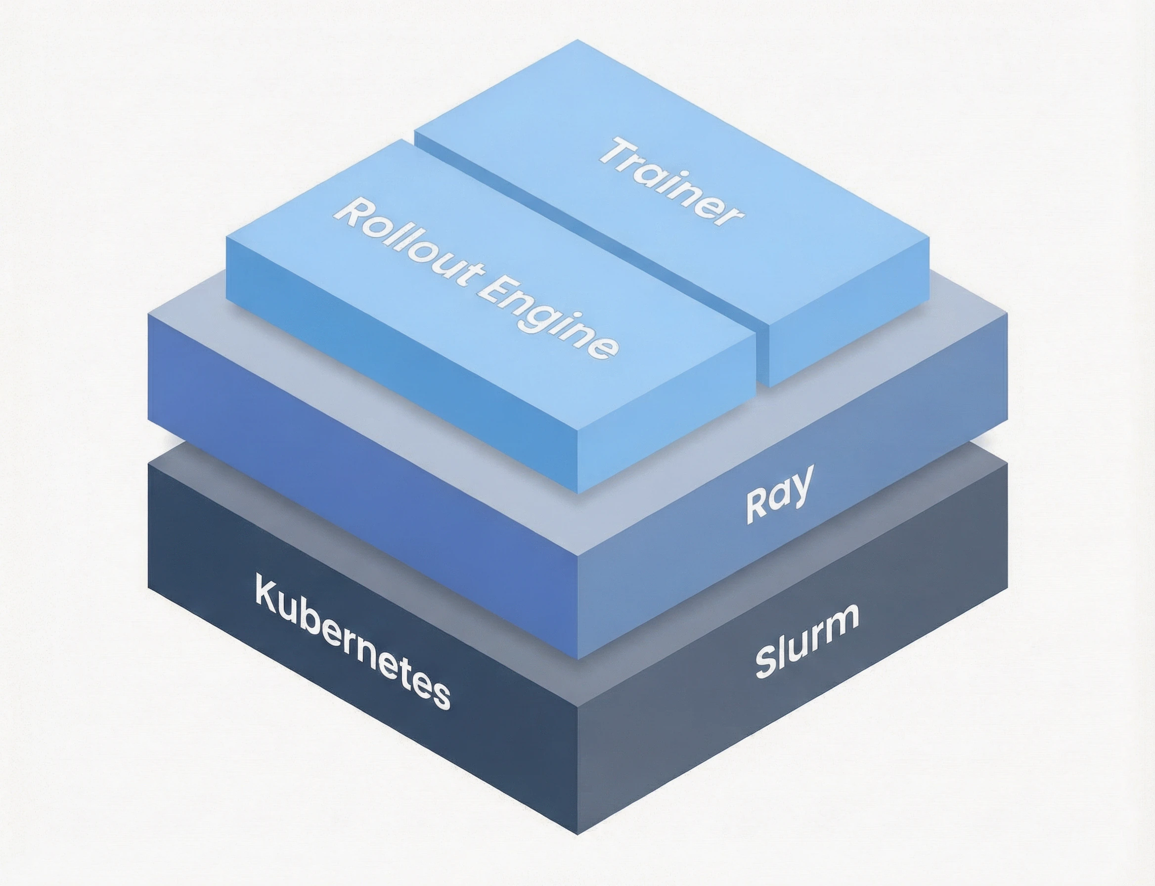
But you don't do it on a bare-bones cluster of nodes connected to a master node via SSH tunneling only. As adults we roll out proper software infrastructure, which might look like a combination of Slurm or Kubernetes as a bottom layer, Ray as the next layer, and on the top layer we have our PyTorch ecosystem libraries that do training and rollout inference.

In practice, setting this up looks like the following. You pin a container image with the driver, the PyTorch build, the inference engine and the training framework, because version drift between vLLM and PyTorch is the most common reason a run dies before step one. On Kubernetes, the Ray cluster is typically launched with KubeRay; on Slurm, an sbatch script starts a Ray head on the first node and workers on the rest. On top of Ray sit the RL frameworks - verl, OpenRLHF, NeMo-RL, or TRL for single-node runs. They split the GPUs into roles (rollout, actor, reference, and critic when there is one). After every update, they sync fresh weights from the trainer to the rollout engine over NCCL (RCCL on AMD). Checkpoints go to shared storage, and metrics go to W&B or similar.

Right now CUDA is the go-to option: most of this stack is built and tested on NVIDIA first. You get prebuilt wheels for flash-attention, vLLM, DeepSpeed and the custom kernels, plus plenty of example configs and issues already solved by someone else. ROCm has caught up a lot. PyTorch, vLLM and SGLang ship ROCm builds, and AMD publishes ready-made Docker images (rocm/pytorch, rocm/vllm). Still, expect to spend some time matching versions and checking that a given kernel or feature is supported, rather than just pip install-ing everything.

Almost Conclusion. Wait why only LLMs?

And it is not limited to LLMs - exactly. Generative models can all be trained with RL.

VLMs - vision language models: one of the features of such models is that they can caption what is depicted in an image, and the location and the relationships of objects can be described in natural language. So it's aligned with the dataset and rl environments used during the training, and highly likely aligned with human perception in general. If we want the model to have a superior level of attention to detail or to deriving assumptions, we might train it with our own data and environments.

Image and video generation - you can do preference optimization (remember RLHF?) by maximizing a reward (a stand-in for human preference) while staying close to a reference model via a KL penalty. Just by showing what a good image or video looks like in your case.

Image editing - this one is harder because one needs before-and-after pairs, which one can only get with labor-intensive labelling.

Audio models - collect human feedback. Users were shown two clips for the same prompt and picked the one they preferred, which produced about 300k pairwise preferences. Train a reward model on those pairs to predict "how much would a human like this clip?" This is what the MusicRL paper does.

Conclusions

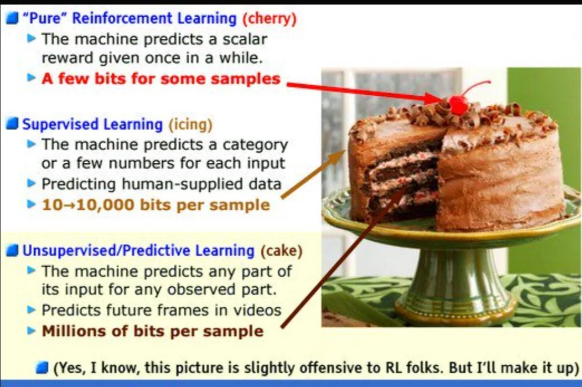
Reinforcement Learning is multifaceted and has been known for a long time; it is extremely pleasant to notice it bringing fruit to hot topics such as auto-regressive language models and image generation. It's worth keeping in mind that RL is the cherry on the pie, meaning it can only do so much in comparison to unsupervised learning and supervised learning. But who knows, perhaps Yann LeCun has been wrong all along? Here's the slide from a famous Yann LeCun talk on the topic.

Thank you for reading!